 |
|
|
| Home | Magnet | Notes | Meetings | Subsystems | Search |
| ||||||||||
|
LHCb Magnet Technical Design Report
Magnet Design Team W. Flegel (Project Coordinator), M. Losasso, F. Rohner CERN
ISBN 92-9083-157-0
Members of the LHCb Collaboration
Univ. of Rio de Janeiro, UFRJ, Brasil S.Amato, D.Carvalho, T.da Silva, J.R.T.de Mello, L.de Paula, F.Galvez-Durand, M.Gandelman, J.Helder Lopes, B.Marechal, L.Martinelli, J.Montenegro, D.Moraes, E.Polycarpo Espoo Vantaa Inst. of Technology, Espoo, Finland O.Bouianov, M.Bouianova, T.Lepola Univ. of Clermont-Ferrand II, France Z.Ajaltouni, G.Bohner, V.Breton, A.Falvard, J.Lecoq, P.Perret, C.Trouilleau, A.Ziad CPPM Marseille, France E.Aslanides, B.Dinkespiler, R.Legac, O.Leroy, M.Menouni, R.Potheau, A.Tsaregorodtsev Univ. of Paris-Sud, LAL Orsay, France G.Barrand, C.Beigbeder-Beau, D.Breton, T.Caceres, O.Callot, Ph.Cros, B.D'Almagne, B.Delcourt, F.Fulda Quenzer, A.Hrisoho, B.Jean-Marie, J.Lefrançois, V.Tocut Humboldt Univ., Berlin, Germany T.Lohse Techn. Univ. of Dresden, Germany R.Schwierz, B.Spaan Univ. of Freiburg, Germany H.Fischer, J.Franz, F.H.Heinsius, K.Königsmann, H.Schmitt Max-Planck-Inst. für Kernphysik, Heidelberg, Germany C.Bauer, D.Baumeister, N.Bulian, H.P.Fuchs, T.Gleber, W.Hofmann, K.T.Knoepfle, M.Schmelling, E.Sexauer, U.Trunk Physikalisches Inst., University of Heidelberg, Germany P.Bock, F.Eisele, M.Feuerstack-Raible, S.Henneberger, P.Igo-Kemenes, C.Richter, P.Schleper Kirchhoff Inst. for Physics, University of Heidelberg, Germany V.Lindenstruth, A.Walsch
Univ. of Bologna and INFN, Italy A.Bertin, M.Bruschi, M.Capponi, I.D'Antone, S.Castro, R.Dona, D.Galli, B.Giacobbe, U.Marconi, I.Massa, M.Piccinini, M.Poli, N.Cesari, R.Spighi, V.Vagnoni, S.Vecchi, M.Villa, A.Vitale, A.Zoccoli Univ. of Cagliari and INFN, Italy M.Caria, A.Lai, B.Saitta Univ. of Ferrara and INFN, Italy V.Carassiti, A.Cotta Ramusino, P.Dalpiaz, A.Gianoli, M.Martini, F.Petrucci, M.Savrie Univ. of Florence and INFN, Italy M. Calvetti, G.Passaleva Univ. of Genoa and INFN, Italy F.Fontanelli, V.Gracco, A.Petrolini, M.Sannino Univ. of Milano and INFN, Italy M. Calvi, C.Matteuzzi, P.Negri, M.Paganoni, R.Pengo, T.Tabarelli de Fatis, V.Verzi Univ. of Rome, "La Sapienza" and INFN, Italy G.Auriemma, L.Benussi, C.Bosio, A.Frenkel, I.Kreslo, S.Mari, G.Martellotti, S.Martinez, M.R.Mondardini, G.Penso, C.Satriano, V.Bocci Univ. of Rome, "Tor Vergata" and INFN, Italy M.Adinolfi, G.Carboni, R.Messi, L.Paoluzi, E.Santovetti
NIKHEF, The Netherlands T.S.Bauer, M.Doets, M.Ferro-Luzzi, R.Hierck, L.Hommels, T.Ketel, B.Koene, M.Merk**, M.Needham, W.Ruckstuhl*, T.Sluijk, O.Steinkamp, W.van Amersfoort, G.van Apeldoorn, N.van Bakel, J.van den Brand, R.van der Eijk, L.Wiggers, N.Zaitsev*** Foundation of Fundamental Research of Matter in the Netherlands, Free University Amsterdam, University of Amsterdam, University of Utrecht, * Deceased; ** Supported by the Royal Netherlands Academy of Science KNAW; ***On leave from St. Petersburg.
Inst. of High Energy Physics, Beijing, P.R.C. C.Jiang, C.Gao, H.Sun, Z.Zhu Univ. of Science and Technology of China, Hefei, P.R.C. G.Jin, X.Lin, T.K.Liu, X. Y.Wu, Z.J.Yin, X.Yu Univ. of Nanjing, Nanjing, P.R.C. D.T.Gao, Z.X.Sha, D.X.Xi, N.G.Yao, Z.W.Zhang
Univ. of Shandong, P.R.C. M.He, X.B.Ji, J.Y.Li, X.Y.Zhang, X.Zhao Inst. of Nuclear Physics, Krakow, Poland E.Banas, J.Blocki, K.Galuszka, P.Jalocha, P.Kapusta, B.Kisielewski, T.Lesiak, J.Michalowski, B.Muryn, Z.Natkaniec, W.Ostrowicz, G.Polok, M.Stodulski, M.Witek, P.Zychowski Soltan Inst. for Nuclear Physics, Warsaw, Poland M.Adamus, A.Chlopik, Z.Guzik, A.Nawrot, M.Szczekowski Inst. of Atomic Physics, Bucharest-Magurel, Romania D.V.Anghel, C.Coca, D.Dumitru, G.Giolu, M.L.Ion, C.Magureanu, S.Popescu, T.Preda, A.M.Rosca, V.L.Rusu Inst. for Nuclear Research (INR), Moscow, Russia V.Bolotov, S.Filippov, J.Gavrilov, E.Guschin, V.Kloubov, L.Kravchuk, S.Laptev, V.Laptev, V.Postoev, A.Sadovski, I.Semeniouk Inst. of Theoretical and Experimental Physics (ITEP), Moscow, Russia S.Barsuk, I.Belyaev, A.Golutvin, O.Gouchtchine, V.Kiritchenko, G.Kostina, N.Levitski, P.Pakhlov, D.Roussinov, V.Rusinov, S.Semenov, A.Soldatov, E.Tarkovski Lebedev Physical Inst., Moscow, Russia Yu.Alexandrov, V.Baskov, L.Gorbov, B.Govorkov, V.Kim, P.Netchaeva, V.Polianski, L.Shtarkov, A.Verdi, M.Zavertiaev Inst. for High Energy Physics (IHEP-Serpukhov), Protvino, Russia I.V.Ajinenko, R.I.Dzhelyadin, A.V.Dorokhov, A.Kobelev, A.K.Konoplyannikov, A.K.Likhoded, V.D.Matveev, V.Novikov, V.F.Obraztsov, A.P.Ostankov, V.A.Polyakov, V.I.Rykalin, V.K.Semenov, M.M.Shapkin, N.Smirnov, M.M.Soldatov, V.V.Talanov, O.P.Yushchenko
St. Petersburg Nuclear Physics Inst., Gatchina, Russia A.Atamanchuk, V.Borkowski, B.Botchine, V.Golovtsov, A.Kashchuk, L.Kudin, V.Lazarev, V.Polyakov, B.Razmyslovich, N.Saguidova, V.Sarantsev, E.Spiridenkov, A.Vorobyov, An.Vorobyov Univ. of Barcelona, Spain P.Conde, L.Garrido Beltran, D.Gascon, R.Miquel, D.Peralta-Rodriguez Univ. of Santiago de Compostela, Spain B.Adeva, F.Gomez, A.Iglesias, A.Lopez-Aguera, M.Plo, J.M.Rodriguez, J.J.Saborido, M.J.Tobar
Univ. of Lausanne, Switzerland P.Bartalini, A.Bay, C.Currat, O.Dormond, Y.Ermoline, R.Frei, J.P.Hertig, P.Koppenburg, J.R.Moser, J.P.Perroud, F.Ronga, O.Schneider, D.Steele, L.Studer, M.Tareb, M.T.Tran Univ. of Zürich , Switzerland E.Holzschuh, P.Sievers, O.Steinkamp, U.Straumann, M. Ziegler Inst. of Physics and Techniques, Kharkiv, Ukraine S.Maznichenko, O.Omelaenko, Yu.Ranyuk, M.V.Sosipatorow Inst. for Nuclear Research, Kiev, Ukraine V.Aushev, V.Kiva, I.Kolomiets, Yu.Pavlenko, V.Pugatch, Yu.Vasiliev, V.Zerkin Univ. of Bristol, U.K. N.Brook, R.Head, F.Wilson Univ. of Cambridge, U.K. V.Gibson, S.G.Katvars, C.Shepherd-Themistocleous, C.P.Ward, S.A.Wotton Rutherford Appleton Lab., Chilton, UK C.A.J.Brew, C.J.Densham, J.G.V.Guy, J.V.Morris, G.N.Patrick Univ. of Edinburgh, U.K. R.Bernet, S.Eisenhardt, F. Muheim, S.Playfer Univ. of Glasgow, U.K. S.Easo, A.J.Flavell, V.O'Shea, P.Teixeira-Dias
Univ. of Liverpool, U.K. S.Biagi, T.Bowcock, P.Hayman, M.McCubbin, G.Patel, D.Wells, V.Wright Imperial College, London, U.K G.J.Barber, P.Dauncey, A.Duane, J.Hassard, M.J.John, J.Lidbury, J.G.McEwen, D.R.Price, B.Simmons, L.Toudup Univ. of Oxford, U.K J.Bibby, N.Harnew, J.Holt, J.F. Libby, I.McArthur, J.Rademacker, N.J.Smale, S.Topp-Jorgensen, G.Wilkinson Univ. of Virginia, Charlottesville, VA, USA S.Conetti, B.Cox, E.C.Dukes, K.S.Nelson, B.Norum Northwestern Univ., Evanston, IL, USA D.Joffe, T.Pedlar, J.Rosen, K. Seth, A. Tomaradze
Rice Univ., Houston, TX, USA D.Crosetto
CERN, Geneva, Switzerland M.Alemi, F.Anghinolfi, A.Augustinus, P.Binko, A.Braem, J.Buytaert, M.Campbell, A.Cass, F.Cataneo, M.Cattaneo, P.Charpentier, E.Chesi, J.Christiansen, R.Chytracek, J.Closier, P.Colrain, O.Cooke, G.Corti, C.D'Ambrosio, H.Dijkstra, J.P.Dufey, F.Filthaut, W.Flegel, F.Formenti, R.Forty, M.Frank, I.Garcia Alfonso, C.Gaspar, A.Go, P.Gras, T.Gys, F.Hahn, S.Haider, A.Halley1, F.Harris, J.Harvey, H.J.Hilke, A.Jacholkowska2, P.Jarron, C.Joram, B.Jost, M.Koratzinos, I.Korolko3, D.Lacarrère, J.Lamas Valverde, M.Laub, F.Lemeilleur, M.Letheren, R.Lindner, M.Losasso, P.Maley, M.Marin, P.Mato, H.Müller, T.Nakada4, J.Niewold, C.Parkes, S.Probst, F.Ranjard, W.Riegler, F.Rohner, T.Ruf, S.Saladino, B.Schmidt, T.Schneider, A.Schöning, A.Schopper, W.Snoeys, W.Tejessy, F.Teubert, I.R.Tomalin, O.Ullaland, E.van Herwijnen, I.Videau2, G.von Holtey, P.Wicht, A.Wright, K.Wyllie, D.Websdale5, P.Wertelaers 1 On leave from Univ. of Glasgow; 2 on leave from LAL, Orsay; 3 on leave from ITEP, Moscow;4 on leave from PSI, Villigen; 5 on leave from Imperial College, London
Members from Non-Participating Institutes J.Seguinot, T.Ypsilantis
Acknowledgements The Magnet Design Team and the LHCb Collaboration are greatly indebted to
Contents
1. Introduction 2. Dipole Design 2.1 Overview 2.2 Coils 2.2.1 Coil Construction 2.2.2 Tests before and during Coil Manufacture 2.3 Yoke 2.3.1 Yoke Construction 2.3.2 Mechanical Tolerances and Magnetic Properties 3. Field Calculations 3.1 Analysis Models in TOSCA and ANSYS 3.2 Field Profiles, Integrals and Uniformity 3.3 Fringe Fields 3.4 Analysis of Forces and Stored Energy 4. Magnet Assembly 5. Electricity and Cooling Requirements 6. Controls System 7. Safety 7.1 General Safety7.2 Mechanical Safety 7.3 Electrical Safety 7.4 Safety in Magnetic Fields 8. Technical Tests at CERN 9. Schedule 10. Cost Estimate and Spending Profile
References
Table 1: Magnet Characteristics
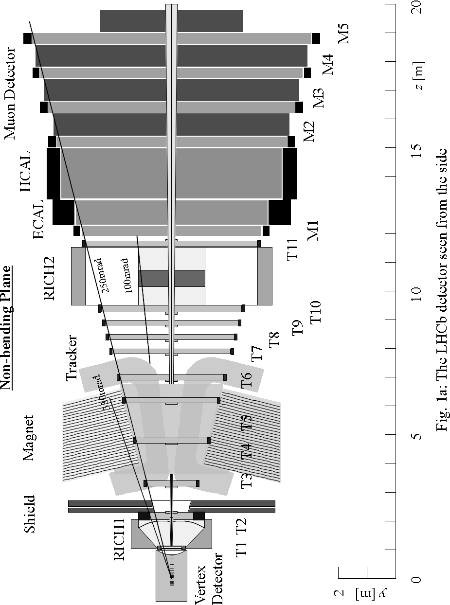
1. Introduction LHCb is an experiment at the Large Hadron Collider (LHC) at CERN to provide precision measurements of CP violation and rare decays in the B-meson system. The high centre of mass energy and luminosity of the LHC combined with the efficient trigger of the experiment, including on-line detection of secondary vertices, will give unprecedented statistics for many physics channels. Particle identification will significantly add to the power of the experiment. The physics goals and details of the detector design are described in the Technical Proposal [1-1]. LHCb exploits the forward region of the pp collisions and requires a dipole field with a free aperture of ±300 mrad horizontally and ±250 mrad vertically. Tracking detectors in and near the magnetic field have to provide momentum measurement for charged particles with a precision of about 0.4% for momenta up to 200 GeV/c. This demands an integrated field of 4 Tm for tracks originating near the primary interaction point. A good field uniformity along the transverse co-ordinate is required by the muon trigger. The lateral aperture of the magnet is defined by the longitudinal extension of the detectors, placed upstream of the magnet. A view of the detector layout is shown in Fig. 1a and 1b. The experiment will be installed in pit 8 of the LEP collider, the cavern presently occupied by the DELPHI detector. For the Technical Proposal a window-frame magnet with superconducting bedstead coils and horizontal pole faces had been assumed, based on a conceptual design from PSI [1-2]. Contacts with industry revealed that the complicated shape of the coils and the high magnetic forces of around 170 ton/m would lead to high cost and mechanical risks. LHCb has, therefore, moved to the design of a warm magnet. To reduce electrical power requirements to about 4.2 MW, the pole faces are shaped to follow the acceptance angles of the experiment. For the same field integral of 4 Tm, the pole face inclination introduces significantly higher fields near the entrance window. The effects of this increased field on the tracking chamber performance and on several physics channels have been studied in detail [1-3]. The effects on physics performance turned out to be weak. In the external sections of two of the tracking chambers the time window of drift signal detection is increased significantly but stays within the accepted limit of 50 ns. Besides the warm magnet described in this report, the option of a superconducting magnet of the same pole face geometry, but with simpler 'race-track' coils has been studied. The conclusion of this comparative study is unambiguous: besides significantly lower costs (the break-even point for construction and operation costs lies beyond 10 years of operation), faster construction and lower risks, the warm coils offer additional advantages, which are very important for LHCb. A warm dipole permits rapid ramping-up of the field, synchronous to the ramping-up of LHC magnets, as well as regular field inversions. The LHCb Collaboration, therefore, adopted a warm dipole magnet. This choice was fully supported by the Magnet Advisory Group MAG of the LHCC [1-4].
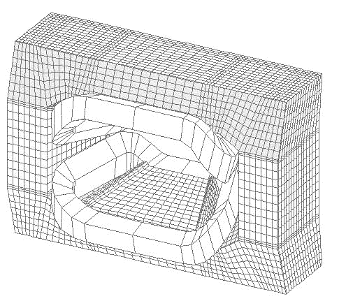
2. Dipole Design 2.1 Overview Various coil shapes and yoke geometries have been studied, including simple race-track designs [2-1], leading finally to the design sketched in Fig. 2.1.1, as viewed from the larger aperture side of the magnet. A photo of a 1:25 model is shown on the cover page. 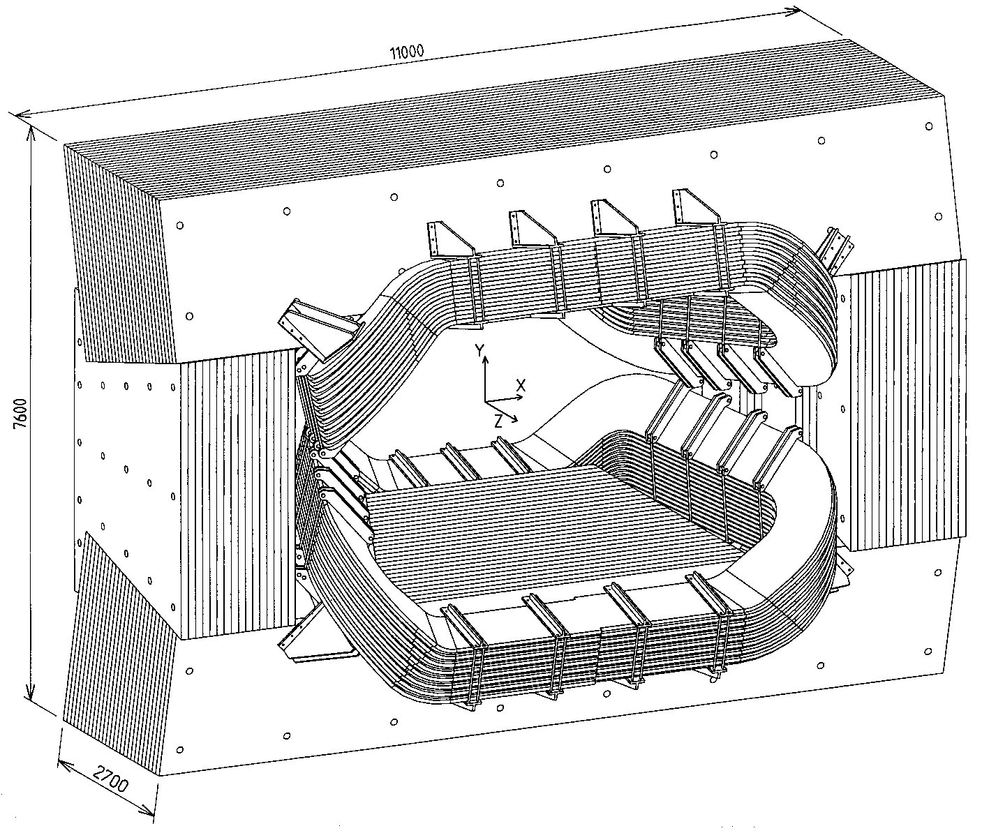
Fig. 2.1.1: Perspective view (EUCLID), without shims The magnet consists of two trapezoidal coils bent at 45° on the two transverse sides, arranged inside an iron yoke of window-frame configuration. The magnet gap is wedge shaped in both vertical and horizontal planes, following the detector acceptance. In order to provide space for the frames of the tracking chambers positioned inside the magnet, the planes of the pole faces lie 100 mm outside the ± 250 mrad vertical acceptance and the shims on the sides of the pole faces 100 mm outside the ± 300 mrad horizontal acceptance. The horizontal upstream and downstream parts of the coils are mounted such that their clamps and supports do not penetrate into the clearance cone defined above for the frames of the tracking chambers. The coils are composed of individual pancakes, which will be connected hydraulically in parallel and electrically in series. The coils have been designed such that enough space is available in the horizontal aperture to maintain and exchange the electronics of the tracking chambers. The iron yoke will be assembled from low carbon steel plates of 80 to 100 mm thickness. We choose a right-handed co-ordinate system with the origin at the interaction point and the z-axis along the beam direction, pointing towards the muon system; the y-axis points upward and x horizontally (see Fig. 2.1.1). The symmetry axes of the dipole follow the same directions, with the principal field component lying along y. The line connecting the centres of the pole faces passes through z = 5.3 m. The principal magnet parameters are listed in Table 1 (page xii). The value of the current given in this table is about 8% higher than the value required for a bending power of 4 Tm (integrated from z = 0 to z = 10 m), according to 3-D calculations with TOSCA (see Section 3). This is to allow a safety factor to cover packing uncertainty due to deviations from flatness of the steel plates. The values for the B-H relation in the TOSCA calculations were taken from a measurement of a steel sample of standard quality Fe360B.
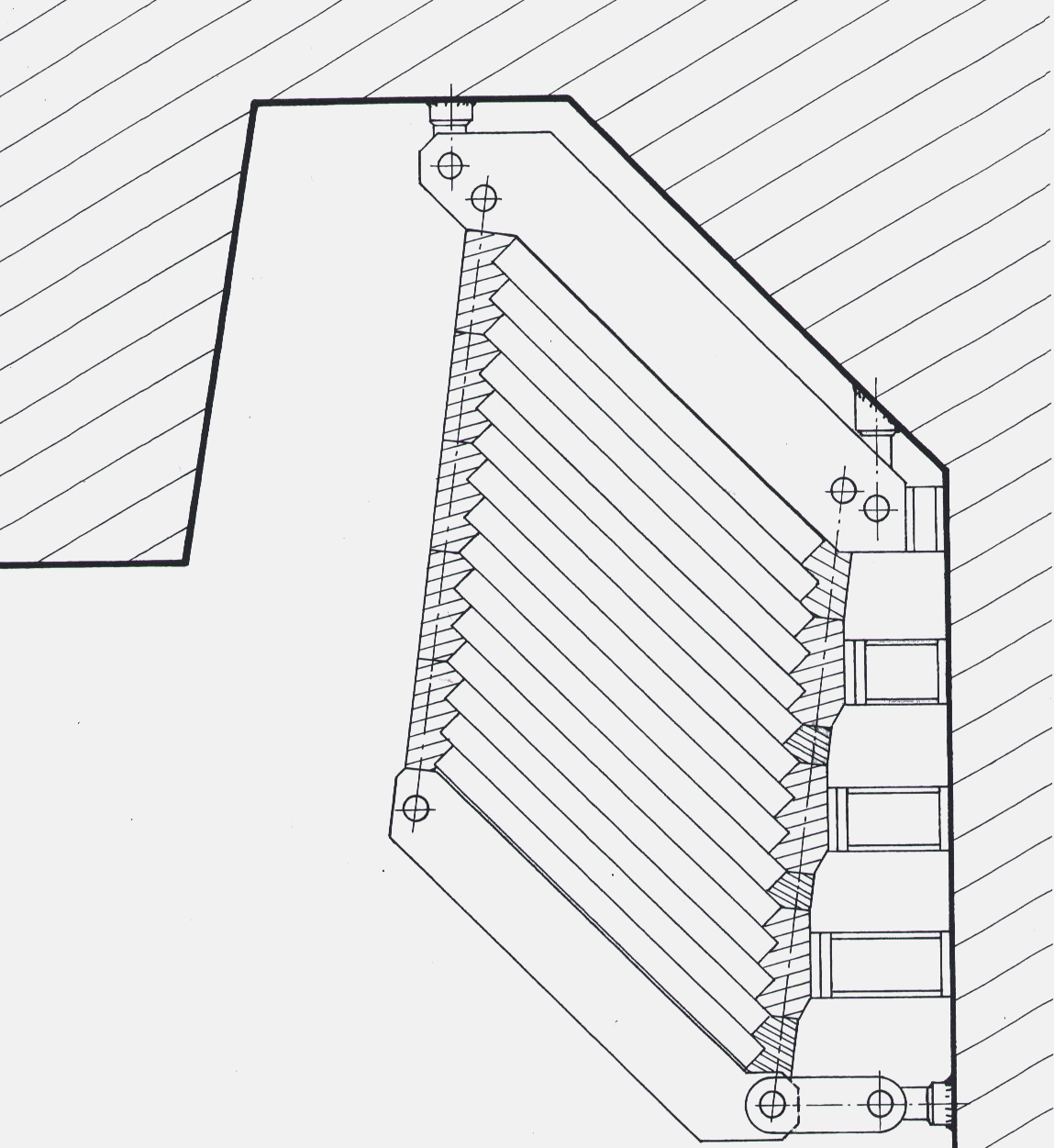
2.2 Coils 2.2.1 Coil construction For reasons of costs and reliability, Aluminium is chosen as conductor material for the coils. A coil is assembled from 15 individual mono-layer pancakes. Each pancake is wound from an extruded conductor of sufficient length to build a mono-layer pancake of 15 turns. No welding is foreseen at the conductor bends of 400 mm radius. The optimum current density for Aluminium coils is usually in the range of 2 to 4 A/mm2. To produce a coil with a high packing fraction of conductor material and to keep the voltage drop across the coil low for safety reasons, it is preferable to use a large conductor cross-section. The design is based on a square conductor of 50 x 50 mm2 cross-section with a central 24 mm diameter bore for water cooling. The four corners will be rounded off with a radius of 3 mm. The conductor will be extruded from pure Aluminium Al-99.7 in an annealed state, having an ohmic resistivity below 28 nW m at 20 ° C. Each pancake will be wound from an extruded single length conductor of about 290 m length. The conductor has to be delivered to the winding facility on spools with a large inner diameter of 2 to 3 m. No damage to the conductor is allowed during its winding onto the spools. In this magnet design all individual pancakes of a coil are of identical trapezoidal race-track shape and wound in the same direction, before being bent by 45° . This allows a serial production of the 2 x 15 pancakes for the two coils without modification of the large motorised winding table. Figure 2.2.1 gives the layout and the principal dimensions of the flat pancake before its bending by 45° .
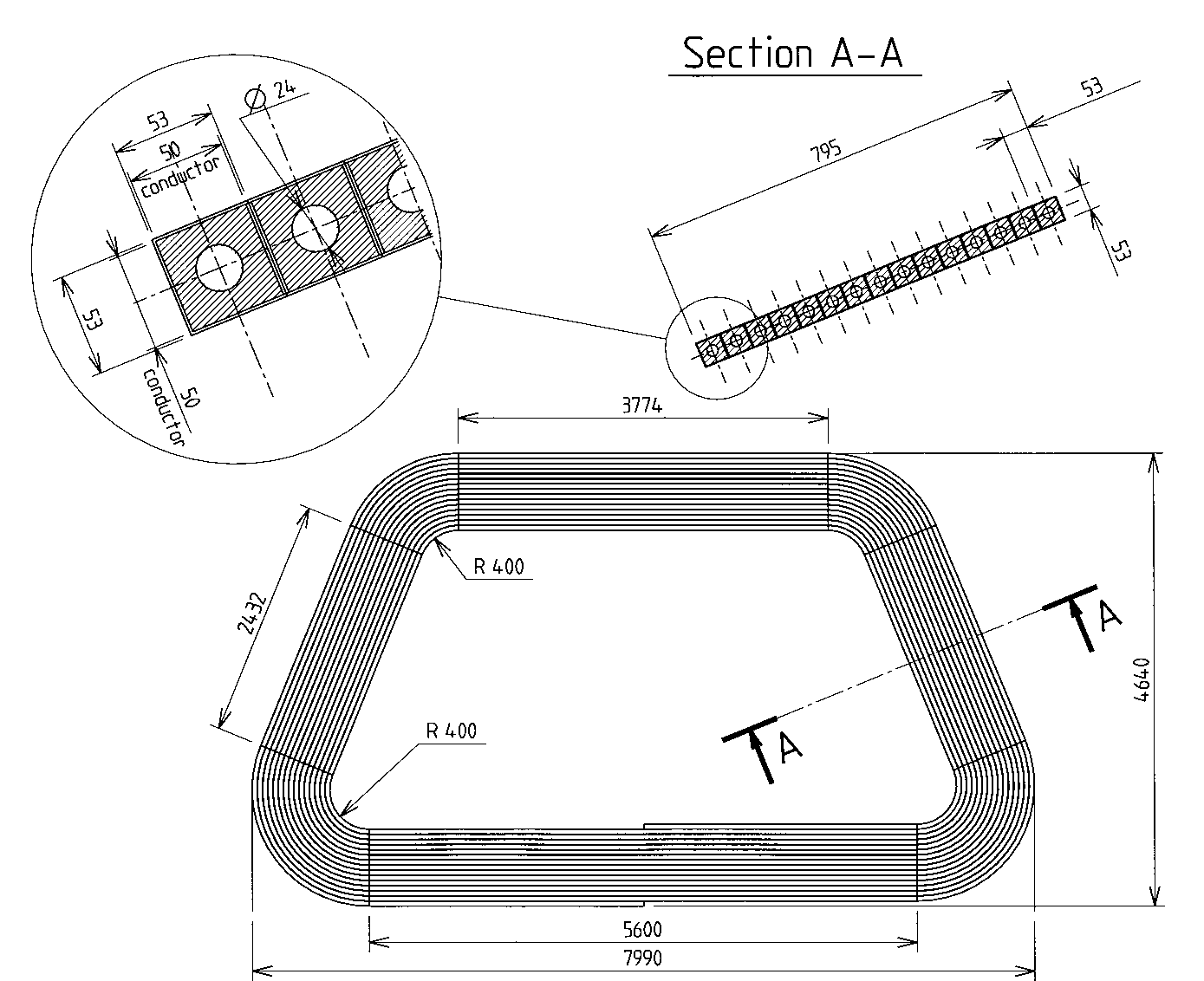
Fig. 2.2.1: Individual pancake (before bending) and its cross-section
The trapezoidal shape of the flat race-track pancakes was chosen such that the two coils after bending by 45° do not touch each other at their smaller gap (upstream) side but are still relatively close to each other at their larger gap (downstream) side. For this reason, the trapezoidal angle is larger than the horizontal aperture of ± 300 mrad and the centre line for the 45° bend is only about 250 mrad. The transversal width of the pancakes was chosen such that the 45º bending does not enter the bend of the conductor at the "corners" of the trapezoidal race-track. The winding of the individual pancakes and their bending by 45° is foreseen to be done without the insulating tape around the conductor. During winding and bending, enough space for the insulation tape and the resin has to be provided by appropriate spacers between neighbouring turns or successive pancakes. The smallest bending radius of 400 mm is rather large to keep the keystone deformation below 3 mm, making possible a subsequent reduction to below 1 mm. This can be done during the winding of the flat pancakes by rolling the conductor between appropriately spaced roller pairs. The roller axis should have an offset angle with respect to the centre of the bend such that the keystone-material is rolled towards the inside of the bend. The 45° bending of the individual pancakes has to be done with a hydraulic press on a special table with variable bending radii depending on the position of the pancakes in the coils. This bend will again produce a keystone deformation of the conductor. Its removal is now more difficult but absolutely necessary to guarantee enough space for the glass fibre tape and the resin. The removal can here be done by grinding. To allow access for the grinding device, the bent pancake turns have to be pulled apart spirally. The pancakes have to be carefully cleaned after removing the keystone deformation. The insulating tape has to be wound around the conductor such that it is half overlapping. This is done after the 45° bending with a small tape winding machine, normally available at the coil manufacturer, to avoid any damage of the insulation during the winding and bending process. To create space for passing the tape winding machine along the conductor, the conductor turns have again to be pulled apart successively, starting at the upper conductor end. Two possibilities for the coil production are considered and will be discussed with industry. In both cases the bending radii for successive pancakes have to be chosen such that no free space between neighbouring pancakes is left after stacking one on top of the other. In the first approach, a coil is assembled from vacuum impregnated and completely finished individual pancakes, separated from each other by two thin Mylar foils. The coil gets its mechanical stability only after the pancakes of the coil are clamped together. These clamps are also used for the transportation of the coil and to support and fix it in the magnet. This arrangement reduces internal mechanical stresses e.g. due to temperature differences. Furthermore each individual pancake can be carefully inspected and tested before coil assembly. In the second approach, the individual glass fibre taped pancakes are stacked together and the coil is vacuum impregnated as one single unit. Its internal mechanical stability is then guaranteed from the beginning. The danger of this approach lies in the volume of the coil, which requires a very careful control of a large amount of resin over a long filling time, to avoid any resin-free pockets. These pockets can not be repaired after the curing of the coil and may lead to coil damage on powering. The rectangular cross-section on the upstream and downstream parts of the coil is skewed on the part bent by 45° . Figure 2.2.2 shows the coil clamps and support structure required to keep the skewed coil section together and to fix it to the yoke, for a coil assembled from individual pancakes. The clamps and supports have to take up the magnetic forces of maximum 94 ton/m (see Section 3.4) and to transmit them to the yoke. Their detailed design is still being optimised. For shortest serial electrical connections between successive pancakes, their winding direction has to be alternating. This can be achieved by either winding half the flat pancakes in the opposite direction or by winding always in the same direction and by turning each second pancake upside down.
Fig. 2.2.2: Coil clamps and support structure
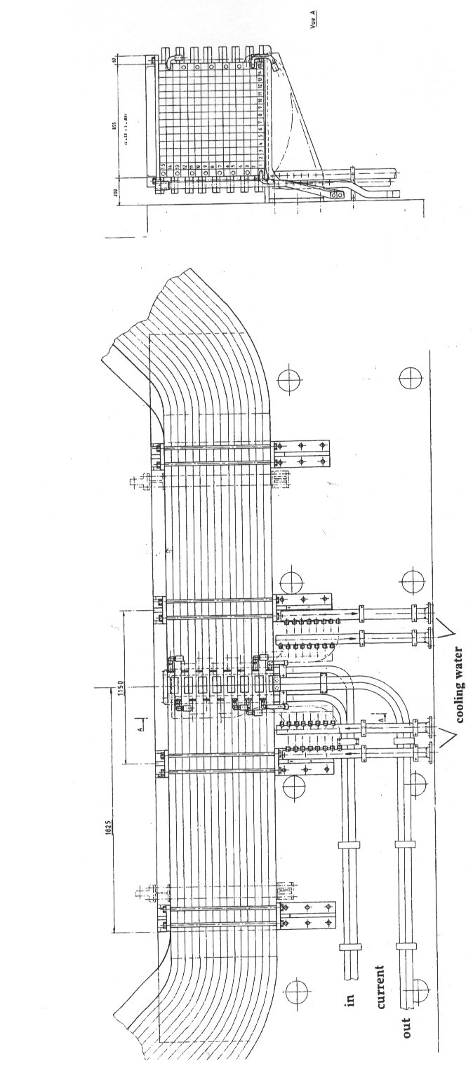
The two coils should then be constructed identically in the sequence of winding directions of the pancakes and their corresponding 45° bend. Each radius setting of the 45° -bending device will be used to produce two identical pancakes, one for each coil. All electrical and hydraulic connections have to be at the downstream side of the magnet because of the space restrictions between coils and shielding plate at the upstream side. All pancakes of the two coils are hydraulically in parallel. To avoid high thermal stresses of the resin at the pancakes, the water inlet for both coils is at the outside. Figure 2.2.3 shows the layout for the electric and hydraulic connections.
Fig. 2.2.3: Layout of the electric and cooling water connections
2.2.2 Tests before and during Coil Manufacture Before extruding the full conductor quantity needed for the coil production, conductor pieces of sufficient length and of the correct cross-section have to be sent to CERN and to the coil manufacturer. These conductor pieces should contain transition sections (extrusion welds) when going from one Aluminium billet in the extrusion press to the next. These sections should be clearly marked. They will be used to test the ohmic resistivity, the mechanical behaviour under high water pressure and under bending, and to optimise the tools and jigs for the pancake winding. The total quantity of conductor required for the two coils should only be produced after successful preparatory tests and an agreement upon the electrical and mechanical properties. The manufacturer has to guarantee these properties for the whole production. The producer has to deliver the conductor to the winding facility on large diameter spools of 2 to 3 m inner diameter, each containing a single length conductor of about 290 m. The coil manufacturer has to guarantee the electrical quality, high voltage insulation and geometrical dimensions of the different pancakes and of the assembled coils. The keystone deformation of the conductor during the winding and bending has to be controlled and removed carefully. The conductor has to be carefully cleaned before being taped with glass fibre tape and vacuum impregnated. The insulation quality turn by turn and turn to ground has to be verified during the whole production process.
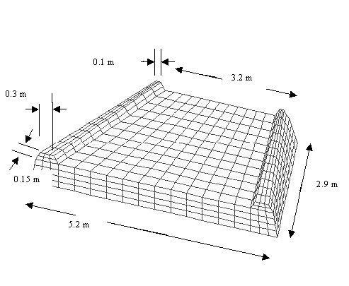
2.3 Yoke 2.3.1 Yoke Construction The magnetic flux generated by the two warm coils is shaped and guided by the iron yoke. It produces a vertical magnetic field in the gap between the pole faces. The yoke consists of two identical horizontal parts including the surfaces of the pole pieces and two identical vertical parts to close the flux return. The horizontal yoke parts are arranged orthogonal to the plane of the coils. This can be seen in the photo of the 1:25 model on the cover page and in the drawing Fig. 2.1.1. Figure 2.3.1 gives a perspective view of only the yoke. The pole pieces are parallel to the vertical aperture of ± 250 mrad with an additional clearance of 100 mm for the frames of the tracker chambers to be installed in the gap. This wedge shape produces higher fields at lower total excitation current than a magnet with horizontal pole faces, for the same field integral of 4 Tm. This reduces the electromagnetic forces on the conductor considerably and leads to acceptable dimensions of the coil cross-section. In the horizontal plane the pole pieces are trapezoidal in shape. Their edges are parallel to the ± 300 mrad aperture but moved outwards by 600 mm to provide 100 mm space for the frames of the tracker chambers and 500 mm for shims. These shims are introduced to enhance the field homogeneity inside the useful horizontal aperture.
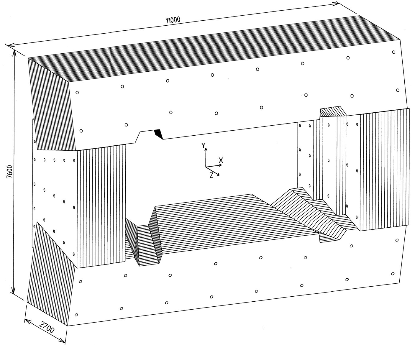
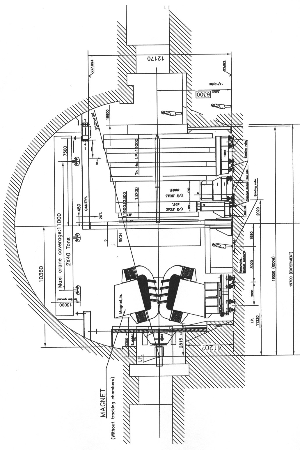
Fig. 2.3.1: Perspective view of the yoke, without shims The coils follow the trapezoidal shape of the pole pieces. This reduces the total conductor length of the coils and thus also the total electrical power consumption. Furthermore, it permits bending of the coils by 45° with only small cut-outs at the horizontal yoke parts. The stronger magnetic field at the upstream side of the aperture requires a larger amount of iron in the horizontal and vertical yoke parts than at the downstream side. This can easily be accommodated in the two vertical yoke parts by having their aperture sides parallel to the cut-outs of the pole pieces in the horizontal yoke and having the outer horizontal and vertical sides of the yoke parallel to the beam axis. The design of the yoke has to respect the boundary conditions given by the existing cavern at pit 8 and its infrastructure. The hall is equipped with two cranes, each of 40 ton lifting capacity and of restricted lateral displacement. For reasons of costs and transportability by road, the magnet yoke parts will be assembled from industrial standard rolled low carbon steel plates of 80 to 100 mm thickness. The maximum weight of a single plate shall not exceed 25 ton. It is intended to re-use the existing rail system, immersed in the concrete floor, to assemble and displace the magnet. Figure 2.3.2 shows a cross-sectional view through the experiment hall with the installation of the LHCb detector, the crane and the rail system.
Fig. 2.3.2: Cross-sectional view of the LHCb detector hall (as seen from the LEP centre).
2.3.2 Mechanical Tolerances and Magnetic Properties
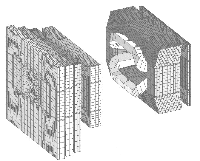
The dimensions of the largest plates for the horizontal yoke part are about 11 m x 2.8 m, and for the vertical one 4 m x 3.1 m. These large dimensions may require that each plate is welded together from two smaller plates. Such welding should be done without affecting the magnetic properties and mechanical tolerances. Welds will have negligible influence on the magnetic properties, when they are performed at the vertical symmetry line of the horizontal yoke plates or along a vertical cut through the vertical yoke plates. Welding the plates together from smaller plates has to be done with minimal gaps and utmost accuracy in order to avoid distortions. Accurate flame cutting with tolerances better than ± 2 mm is acceptable to shape all the plates and to produce the chamfers for welding if needed. Sharp edges and burrs shall be ground off. Rust and scale should be taken off by sandblasting. A thin protective paint is required for all plates. Machining of the plates is necessary at the faces where the horizontal and vertical yoke parts are in contact with each other, and at the two pole faces. In addition, about 16 holes of 90 mm diameter have to be flame-cut or drilled into each plate of the horizontal yoke parts and up to 12 holes into each plate of the vertical yoke parts. These holes will be used to tie the plates of the different yoke parts together by M80 tie-rods. The variation of the plate thickness should be below ± 0.5 mm and the flatness tolerance below 1 mm/m, including the parts which might have been welded. The magnetic induction B at a field of 30 000 A/m must be higher than 2 Tesla and the coercive field must be lower than 240 A/m. These values are normally reached by standard quality steel according to EURONORM EN 10 025 of designation S235JR, also referred under material number 1.0037. (Older designations are Fe360B, St37-2.) Only steel plates of uniform chemical composition and having undergone the same heat treatment will be used. Ring-shaped samples extracted from the manufactured plates and representative for the whole plate supply have to be sent to CERN for measurements of the magnetic properties before delivery of the plates to CERN. 3. Field calculations 3.1 Analysis models in TOSCA and ANSYS The magnet design was assisted by Finite Elements (FE) calculations. First results were obtained in 2-D computations using the POISSON programme. These calculations were followed by full 3-D analysis, mainly with the Vector Fields TOSCA programme, but also with ANSYS. Some of the 3-D field maps were used in the LHCb physics simulation programme to investigate the effects of field geometry and field inhomogeneities on the detector and physics performance. The complete TOSCA 3-D model of the magnet is shown in Fig. 3.1.1. This model was used to study saturation effects in the magnet yoke, field inhomogeneities and field integrals in the tracking volume from z = 0 to z = 10 m and to derive stray field estimates in the region of the first Ring Imaging Cherenkov counter (RICH1). It contains at the upstream side of the magnet two shielding plates to reduce the stray field in the volume around the RICH1 photo-detectors. The first shielding plate, shown in Fig. 3.1.4 starts at z = 2300 mm (just downstream of RICH1) and is 150 mm thick. The second one starts after a gap of 50 mm at z = 2500 mm, and is 200 mm thick.
Fig. 3.1.1: TOSCA model All TOSCA computations used the measured B-H relationship of the iron, while the packing factor of the laminated iron yoke was taken as 1. A physics simulation was carried out using a field map generated with the TOSCA model shown above, on a grid spacing of 10 cm in a volume of about 4 m x 4 m x 14 m (horizontal, vertical, axial directions). This field map includes the two iron shields in the upstream region, but not the iron of the hadron calorimeter and of the muon system. The geometry of the pole shims was roughly optimised using the POISSON programme. The segmentation used in the FE analysis is shown in Fig. 3.1.2.
Fig. 3.1.2: Shimmed pole used for TOSCA models
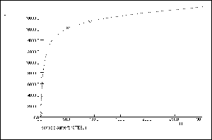
The dependence of the field on the iron properties has been evaluated. For iron specifications ranging from very high to normal commercial quality 0.2% Carbon content, no major effect has been found on any important parameter. We have, therefore, decided to use standard quality steel, whose designation is S235JR according to Euronorm EN 10025. The B-H curve used for the analysis is shown in Fig. 3.1.3. In order to compute the downstream stray field in the region of RICH2 and the muon chambers, the model was extended from z = - 4 m up to z = 21 m, including the structured iron of the hadron calorimeter and the block walls of the muon filter. This new model is shown in Fig. 3.1.4. The number of nodes for this latter model is approximately 265000, and the limit is about 25 m along z and 24 m along the other two dimensions. The change in the integral of the vertical component of the magnetic field computed over 10 m along the beam direction, is negligible (less than 0.1%) when computed with or without the iron of the hadron calorimeter and of the muon shields.
Fig. 3.1.3: B-H curve for Fe360. (Units are Gauss and Oersted)
Fig. 3.1.4: TOSCA model with hadron calorimeter and muon shields
3.2 Field Profiles, Integrals and Uniformity
The measure of field uniformity of greatest relevance to the experiment is the uniformity of the integral of the principal component, By, evaluated along straight tracks originating at the interaction point. Table 3.2 summarises the field integrals from z = 0 to z = 10 m for a central track and for three tracks near the acceptance boundary. The variations relative to the central track are below 6%. Table 3.2: Field integrals along selected tracks
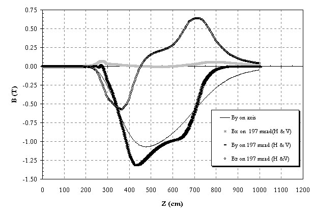
The variation of the vertical field component, By,
along the beam direction is shown in Fig. 3.2.1 for a central track and one for
197 mrad (in x and y). For comparison with Fig. 5.8 of the Technical Proposal
also Bx and Bz along 197 mrad are shown. A current of 1.2
MA per coil has been assumed. As the field uniformity is strongly dependent on
the geometry of the pole shims, further optimisation is possible. Fig. 3.2.1: Magnetic field along selected tracks.
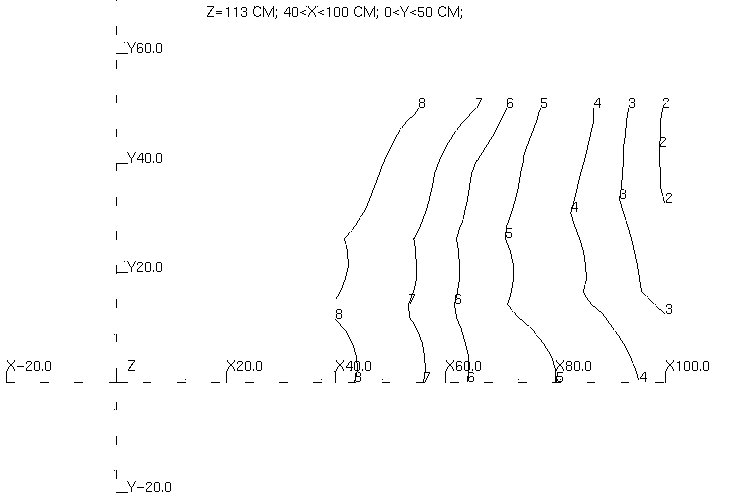
3.3 Fringe Fields In order to reduce the fringe field in the upstream region, two iron shields are added, separated by a 50 mm air gap. The first shield extends from z = 2300 mm to z = 2450 mm, the second plate from z = 2500 mm to z = 2700 mm. The conical apertures in the shields are along 270 mrad in the vertical direction and 300 mrad in the horizontal one. The field in the region of the photo-detectors of RICH1 is below 50 Gauss. Fig.3.3.1 shows a field map at z = 1130 mm from the origin.
Fig. 3.3.1: Fringe field at z = 1130 mm, in the region of RICH1 photo-detectors. Isolines are drawn for field values, ranging from 29 Gauss (line 2) to 36 Gauss (line 8). Co-ordinates in cm.
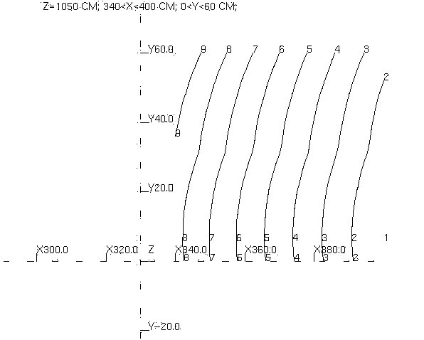
In the RICH2 region, the fringe field has been evaluated with an approximated description of the iron absorbers of the hadron calorimeter and the muon detector. Fig. 3.3.2 shows a field map at z = 10500 mm in the x-y plane.
Fig. 3.3.2: Fringe field at z = 10500 mm, in the region of RICH2 photo-detectors. Isolines are drawn for field values ranging from 99 Gauss (line 2) to 146 Gauss (line 9). Co-ordinates in cm.
The accuracy of these numbers is limited by the number of mesh points used, the approximation for the iron layout in the detectors and by undefined additional iron nearby (e.g. from the crane or from the reinforced concrete walls). It is planned to install the magnet early enough to be able to carry out measurements, which will allow to optimise the magnetic screening of the photo-detectors for both RICH detectors.
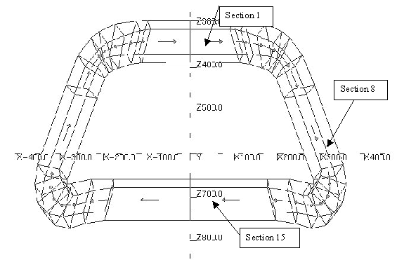
3.4 Analysis of Forces and Stored Energy For the 3-D field and force analysis with TOSCA, the coil was modelled with 30 brick conductors. The body force on the individual source conductors was computed using J x B. Table 3.4.1 summarises the force components for the 15 bricks forming one half of the upper coil. The convention used is indicated in Fig. 3.4.1.
Fig. 3.4.1: Definition of coil sections
Table 3.4.1: Lorentz forces on coil sections (upper coil)
The forces acting on the shielding plates and the iron blocks of the detector are given in Table 3.4.2; they are computed by integrating the Maxwell stress tensor over the surfaces under consideration. Due to the symmetry of the problem, only the component along the z direction has to be considered. The forces on the detector iron turn out to be only a small fraction of the gravitational loads. The forces on the shielding plates are transmitted via beams to the magnet yoke.
Table 3.4.2: Magnetic forces on detector parts
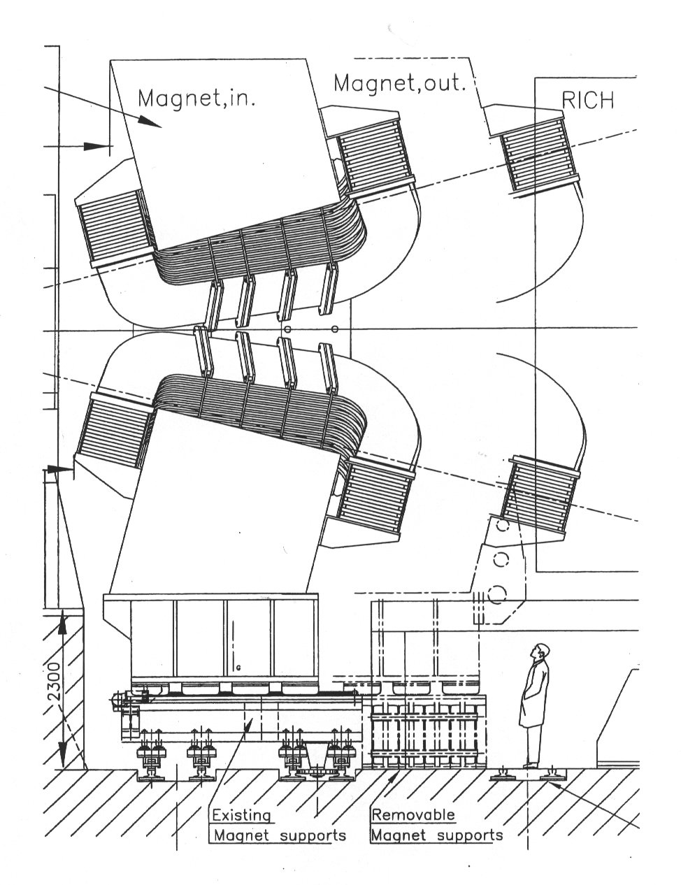
4. Magnet Assembly The position of the magnet in the experiment is outside the crane coverage. The magnet has therefore to be assembled in an area reachable by the crane before being rolled into its final position. It is foreseen to re-use the DELPHI magnet carriage on its rail system as platform for the magnet. The assembly position (magnet out) and the final position (magnet in) of the magnet are indicated in Fig. 4.1.
Fig. 4.1: Magnet position during assembly
With the carriage below the crane, the following sequence has to be observed. The smallest plate of the lower horizontal yoke part will be fixed against a temporary support mounted onto the carriage. The next larger plates will be placed against each other. Before tensioning the tie-rods, which keep the yoke plates solidly together, the individual iron plates have to be adjusted in height with wedges such that the two surfaces, which will be in contact with the vertical yokes, are in a plane. Remaining local uneven spots after tensioning of the tie-rods should be shimmed with soft iron pads. The horizontal yoke part should now be solidly supported and fixed to the platform of the carriage. At this moment the shims for the magnet aperture can be fixed to the lower pole-pieces. To mount a vertical yoke part, a lateral support has to be provided, which fixes temporarily the outermost plate in its vertical position, but leaves enough space for mounting the tie-rods. During the assembly, the plates have to be secured against falling over. Having reached the correct number of sheets for each thickness step of the vertical yoke, the corresponding tie-rods will be mounted and pre-stressed. After having mounted all plates of a vertical yoke, the remaining tie-rods will be mounted and all tie-rods stressed. Possible unevenness due to the machining tolerances will mainly show up at the upper machined surface of the vertical yokes. Again they will be shimmed with soft iron strips of proper thickness. Because of the restricted space between coils and yoke plates, the proper contact and functioning of the electric and hydraulic connections and of the control sensors have to be carefully tested before mounting the coils in the magnet. Having mounted the two vertical yoke parts, the lower coil will first be placed into the magnet and provisionally supported in a position as low as possible. The same has to be done with the upper coil. This assures the safe introduction of the lower row of tie-rods in the upper horizontal yoke part. The assembly of the upper yoke part is similar to the lower one, except that it starts with the largest plate. Possible small slits between the contact surfaces of the upper and vertical yoke parts, which might show up after stressing the tie-rods, will again be closed by soft iron strips. The different yoke parts will then be solidly fixed by welded clamping brackets, their relative position to each other being assured by appropriate dowel pins. Only now the two coils, first the upper and then the lower one, will be placed into their final position and solidly fixed with their clamps and supports to the yoke. Starting from the arrival and distribution point at the magnet, the current connections and the cooling water distribution will be mounted and connected to the coils, as indicated in Fig. 2.2.3. After rolling the completed magnet into its final position, the downstream part of the carriage will be removed to make space for other detector supports. The magnet can now be connected to the bus-bar cables from the power supply and to the cooling water port and commissioning may start.
5. Electricity and Cooling Requirements The 3-D field calculations, using a 100% packing density for the yoke and a B-H relation as measured for Fe360B (Section 3.1), require a total excitation current of 2 x 1.2 MA to achieve the field integral of 4 Tm. This leads to an electric power dissipation of 3.54 MW. The nominal value of 4.2 MW, as given in Table 1, is, therefore, considered as a conservative upper limit. It is proposed to place the transformer and power supply into the surface building SUH of the LHC8 area. This results in a distance of about 200 m between power supply and magnet. Using 2 x 12 Cu power cables of 240 mm2 cross-section and 200 m length leads to additional power losses of roughly 2%. The inefficiencies of the transformer and power supply are of the order of few % only. A network power to the transformer of 6 MVA is required. With a total of 8 MW being available for the experiment and about 2 MW being reserved for the detector electronics and computing, these 6 MVA are available for the magnet. Tables 5.1 and 5.2 summarise the electricity and cooling requirements for the magnet and the power supply.
Table 5.1: Magnet requirements
Table 5.2: Power supply requirements
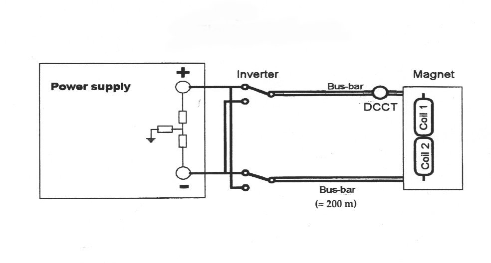
The output voltage of the power supply will be symmetric to ground via an active ground watch circuit according to the IT scheme (IEC364 and IS24 [5-1]). The ground watch circuit switches the power supply off when exceeding a predefined current to ground or at loss of ground reference. Figure 5.1 shows schematically the electrical layout of the power supply and its connection to the magnet.
6. Controls System A detailed magnet controls system to supervise the magnet operation has been worked out in collaboration with the CERN-EP-EOS group and follows the standard elaborated in common for the four LHC experiments [6-1].
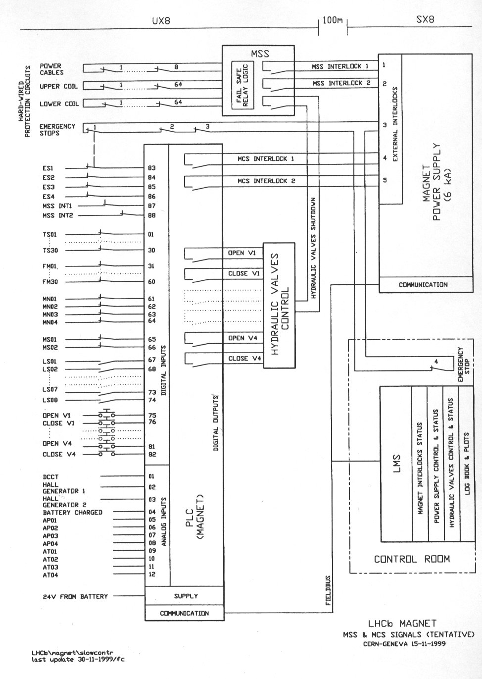
This system, via a net of sensors and actuators, will provide the remote control of power supply and its ground watch circuit, of the inverter, bus-bar, DCCT, cooling water, water leak detector, temperature of coils, fire detector, magnetic field level [6-2]. Figure 6.1 shows the layout of the magnet instrumentation. Table 6.1 explains the abbreviations used in this scheme.
Table 6.1: Naming convention
An integrated system of hardwired interlocks, working according to AND logic, will supervise the safety, e.g. emergency buttons, water leak detection, power supply fault, fire alarms. This system will be interfaced to other LHCb specific systems as well as to the central LHC control room. Figure 6.2 shows its interconnection to the magnet control system.
Fig. 6.1: Layout of the magnet instrumentation
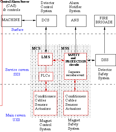
Fig. 6.2: Integration of the interlocks into the Magnet Controls System The Magnet Control System (MCS) is made of two parts:
Interfaces with the other systems CAS, DCS, DSS, ANS are explained in the block diagram Fig. 6-3.
Fig. 6.3: Schematic layout of the Magnet Controls System
The MCS can be accessed by the LHCb experiment or by the Main Control Room of the LHC machine to allow the ramping of the LHCb magnet together with the beam magnets.
7. Safety 7.1 General Safety The general safety is based on the Magnet Safety System (MSS), as part of the Experiment Control System (ECS/DCS). The basic functions of the MSS are defined in Section 6 and [6-1]. The magnet power supply is interlocked to the general fire alarm and to the specific water leak alarm for the magnet. The boxes used for protection against electrical hazards (see Section 7.3) also serve as protection against water spills. These protection boxes are equipped with water leak sensors and are connected to a sink.
7.2 Mechanical Safety All the construction parts, supports and tools required for the assembly will follow European directives, CERN safety codes and rules and the CERN safety policy expressed in the SAPOCO document [7-1]. General criteria for safe stress levels will follow European and/or international structural engineering codes stated in Eurocode-3 [7-2] and AISC [7-3]. For anchoring points, lifting and rigging gears, which will remain the property of CERN/LHCb, the design, manufacture and testing shall comply with the CERN Safety Code on Lifting Equipment (Safety Code D1 [7-4]) and construction normes and codes of ISO and FEM [7-5].
7.3 Electrical Safety The conductor insulation will conform to CERN Safety Instructions IS23 and IS41 [7-6] and will be tested to 3 kV. The power supply will be of the insulated IT-type (IEC364 and IS24 [5-1]), as described in Section 5. Low voltage safety rules will apply according to CERN Safety Instructions IS33 [7-7] and IS24 [5-1]. As protection against electrical hazards, the region of the coils with the electrical interconnections of the pancakes and the coil connection to the bus-bar will be completely surrounded by a polycarbonate (Macrolon) box. This includes also the flexible water connections. Figure 2.2.3 shows the layout of the electric and cooling water connections.
7.4 Safety in Magnetic Fields
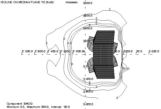
Safety requirements stipulated in CERN Safety Instruction IS36 [7-8] will be respected. The general safety system will be based on the Magnet Safety System (MSS) and the Experiment Control System (ECS/DCS). As the dipole aperture is very large and a large part of the pole pieces is saturated, a strong fringe field is present, up to 20 mT at a distance of 5 m from the iron yoke, as shown in Fig. 7.1. A fence shall be installed delimiting a zone around the magnet with restricted access and with warning lamps blinking, whenever the power on the magnet is switched on. Without circulating beams, this will happen only rarely for special tests. In these cases, access into this zone will have to be specially authorised by the GLIMOS. Continuous work is permitted for authorised persons in zones where the field does not exceed 200 mT (CERN Safety Instruction IS36). For such work the use of non-magnetic tools is mandatory. After any intervention near the magnet with magnetic field switched off, a systematic check will be carried out to free the field volume from ferromagnetic objects, before ramping up the magnet.
Fig. 7.1: Isofield lines in the yz-plane at x = 0 m The separation between two isolines is 10 mT. Isofield line 3 corresponds to 20 mT. Co-ordinates in cm.
8. Technical Tests at CERN To study technical problems related to the coil production, bending tests with modified spare pieces of the UA1 Aluminium conductor will be carried out at CERN. A pancake with final conductor cross-section but smaller lateral dimensions will be wound.
9. Schedule The construction of the warm magnet is not on the critical path for LHCb, in contrast to the option of the superconducting magnet proposed in the Technical Proposal. Nevertheless, an early delivery is important to allow enough time for detailed field measurements and for the optimisation of the magnetic shielding, in particular for the photo-detectors of the two RICH counters. Market surveys have been launched in September 1999, separately for the extrusion of the aluminium conductor (MS-2779/EP/LHCb), the production of the two coils (MS-2773/EP/LHCb) and the yoke (MS-2774/EP/LHCb). The tendering is scheduled for April 2000. Orders should be placed in autumn 2000, assuming this Technical Design Report will be approved by the LHCC and the LHCb Resources Review Board (RRB) authorises Common Fund spending. Delivery of all components should then be possible by end of 2002. Assembly and commissioning of the magnet in Pit 8, as well as the field mapping will be terminated by August 2003. This will avoid any interference with the installation of detector supports and components. Table 9.1 summarises the schedule. It fits well the installation schedule for the experiment. Table 9.1: Magnet Schedule
10. Cost Estimate and Spending Profile Definite costs will only be known after conclusion of the tendering process. It is, however, possible to give crude estimates, based on previous experience with aluminium conductor production and recent offers for iron plates. The cost of the iron plates for the yoke is expected to lie around 4.5 MCHF, the cost for the aluminium extrusion around 0.5 MCHF and for the coil fabrication close to 1 MCHF. The approximate spending profile is shown in Table 10.1.
Table 10.1: Spending Profile
References
[1-1] LHCb Technical Proposal, CERN/LHCC 98-4 [1-2] "Design study of a large-gap superconducting spectrometer dipole", D.C. George, R.K. Maix, V. Vrankovic and J.A. Zichy; LHCb 98-020 [1-3] a) Presentations during the LHCb week in Amsterdam; P. Colrain, R. Forty, R. Hierck, A. Jacholkowska, M. Merk, B. Schmidt, G. Wilkinson, LHCb 99-052 b) "Influence of the new magnet design on tagging"; R. Forty, LHCb 99-010 c) "LHCb Magnet Review Report", B. Koene and J. Lefrançois. Report from the internal referees to the LHCb Technical Board, May 1999 * [1-4] "Resistive magnet for LHCb", T. Taylor, LHCC/99-35 *
[2-1] LHCb 2000-007, in preparation [5-1] International Electrotechnical Commission, directive IEC364, CERN Safety Instruction IS24 (1990): Regulations applicable to electrical installations [6-1] Technical Note EP-EOS-LHCb-01.12.99 [6-2] F. Cataneo, Private Communication [7-1] SAPOCO/42, rev. 1994: Safety Policy at CERN [7-2] Eurocode-3, Design of steel structures (ENV 1993-1-1 edited by Comité Européen de Normalisation) [7-3] AISC-American Institute of Steel Construction, Manual of Steel Construction, Allowable Stress Design, 9th ed., Dec. 1995 [7-4] CERN Safety Code D1, rev. 1996: Lifting Equipment [7-5] ISO-International Standardisation Organisation, FEM-Fédération Européenne de Manutention [7-6] CERN Safety Instruction IS23 rev. 1993: Criteria and standard test methods for the selection of electric cables, wires and insulated parts with respect to fire safety and radiation resistance. CERN Safety Instruction IS41 rev. 1995: The use of plastic and other non-metallic materials at CERN with respect to fire safety and radiation resistance. [7-7] CERN Safety Instruction IS33 rev. 1999: Voltage domains according to IEC [7-8] CERN Safety Instruction IS36 rev. 1993: Safety Rules for the Use of Static Magnetic Fields at CERN * Restricted circulation only
|